Pandas DataFrame in Python is a two dimensional data structure. It means the dataframe stores data in a tabular format i.e., rows and columns.
This article shows how to create a DataFrame, and access, and alter rows and columns. Next, we will discuss Transposing DataFrame in a library, Iterating over rows, and so on.
How to create a pandas DataFrame in Python?
In real-time, we use this Python Pandas dataFrame to load data from SQL Server, Text Files, Excel Files, or any CSV Files. Next, we slice and dice that data as per our requirements. Finally, once the data is in our required format, we use that data to create reports, charts, or graphs using the matplotlib module.
Create an Empty DataFrame in Python pandas
It is a simple example of creating an empty DataFrame. Here, we are creating an empty one.
import pandas as pd

data = pd.DataFrame()
print(data)
Creating an Empty DataFrame output
Columns: []
Index: []
Create Python pandas DataFrame from the List
Here, we create a list of integer values. Next, we used the DataFrame function to create our df from the list or to convert the list.
table = [1, 2, 3, 4, 5]

data = pd.DataFrame(table)
print(data)
   0
0  1
1  2
2  3
3  4
4  5
Creating from a Mixed List or converting a Mixed List to a Pandas Data Frame. Here, we also use multiple rows and columns.
mixedtable = [[1, 'Suresh'], [2, 'Python'], [3, 'Hello']]

mixeddata = pd.DataFrame(mixedtable)
print(mixeddata)
We must use the columns argument to assign the names to column values. For instance, the below code provides names to columns instead of 1 and 2.
mixdata = pd.DataFrame(mixedtable, columns = ['S.No', 'Name'])
print(mixdata)
   0       1
0  1  Suresh
1  2  Python
2  3   Hello

# WIth Names Output
   S.No    Name
0     1  Suresh
1     2  Python
2     3   Hello
Python pandas DataFrame of Random Numbers
To create a DataFrame using random numbers, we used the numpy random function to generate random numbers of size 8 * 4. Next, we used the function to convert those sequences to a DataFrame
import numpy as np
import pandas as pd

d_frame = pd.DataFrame(np.random.randn(8, 4))
print(d_frame)
          0         1         2         3
0 -0.492116 -0.824771 -0.869890 -1.753722
1 -0.733930  0.947616  0.089861  0.888474
2 -0.948483 -1.002449 -0.283761 -0.207897
3  0.013346  2.059951  1.064830  0.830474
4  0.289157 -0.418271 -0.770464  0.223895
5 -0.781827 -0.396441  0.123848 -0.824002
6  0.667090  0.183589  1.212163  0.231251
7  1.067570 -0.615639  0.461147 -1.365541
Python Pandas DataFrame from dict
It allows you to create DataFrame from a dict or dictionary. It was pretty much straightforward. All you have to do is declare a dictionary of different values and then use the function to convert that dictionary to DataFrame.
table = {'name': ['John', 'Mike', 'Suresh', 'Tracy'],
         'Salary':[1000000, 1200000, 900000, 1100000]
         }

data = pd.DataFrame(table)
print(data)
To create a df from dict, all dictionary values should be the same length as all keys. Otherwise, it throws an error. Next, if you pass the index values, they should match the length of key values or arrays; otherwise, it raises an error. Finally, if you haven’t passed any index values, it will automatically create an index for you, starting from 0 to n-1.
name Salary
0 John 1000000
1 Mike 1200000
2 Suresh 900000
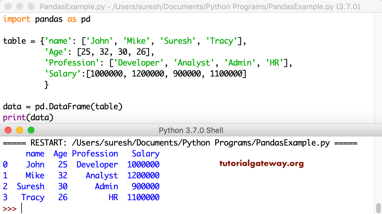
3 Tracy 1100000Let me take another example of DataFrame from Dictionary. This time, we are converting the Python dictionary keys of four columns of Data.
table = {'name': ['John', 'Mike', 'Suresh', 'Tracy'],
         'Age': [25, 32, 30, 26],
         'Profession': ['Developer', 'Analyst', 'Admin', 'HR'],
         'Salary':[1000000, 1200000, 900000, 1100000]
         }

data = pd.DataFrame(table)
print(data)
How to create Python pandas DataFrame from dict of lists
If you are confused about placing everything in one place, divide them into parts. Here, we declared four lists of items and assigned them for each column.
names = ['John', 'Mike', 'Suresh', 'Tracy']
ages =  [25, 32, 30, 26]
Professions = ['Developer', 'Analyst', 'Admin', 'HR']
Salaries = [1000000, 1200000, 900000, 1100000]

table = {'name': names,
         'Age': ages,
         'Profession': Professions,
         'Salary': Salaries
         }

data = pd.DataFrame(table)
print(data)
     name  Age Profession   Salary
0    John   25  Developer  1000000
1    Mike   32    Analyst  1200000
2  Suresh   30      Admin   900000
3   Tracy   26         HR  1100000
DataFrame of Dates
You can also create a DataFrame with a series of dates using this module. For example, let me make one with dates from 2019-01-01 to 2019-01-08. By changing the period values, you can generate more number of Date sequences.
dates = pd.date_range('20190101', periods = 8)
print(dates)
print()

d_frame = pd.DataFrame(np.random.randn(8, 4), index = dates,
                       columns = {'apples', 'oranges', 'kiwis', 'bananas'})
print(d_frame)
DatetimeIndex(['2019-01-01', '2019-01-02', '2019-01-03', '2019-01-04',
               '2019-01-05', '2019-01-06', '2019-01-07', '2019-01-08'],
              dtype='datetime64[ns]', freq='D')

               kiwis    apples   oranges   bananas
2019-01-01 -0.393538 -0.406943  1.612431  1.089230
2019-01-02  1.070080 -1.565538  0.727056  1.677534
2019-01-03 -1.324169  0.256827  1.332544 -2.952971
2019-01-04  0.419778 -0.562119  0.507846 -0.223730
2019-01-05  0.175785  1.566511 -1.832633  2.035536
2019-01-06  0.541516 -0.113477  0.444046  0.387718
2019-01-07  0.247760 -1.143530  0.615681  0.400743
2019-01-08 -0.242328  0.913758 -0.088591 -0.533690
Python pandas DataFrame Columns
This example shows how to reorder the columns. By default, Data Frame will use the column order we used in the actual data. However, you can use this argument to alter the position of any column. For example, let me change the Age from the second position to the fourth position.
table = {'name': ['John', 'Mike', 'Suresh', 'Tracy'],
         'Age': [25, 32, 30, 26],
         'Profession': ['Developer', 'Analyst', 'Admin', 'HR'],
         'Salary':[1000000, 1200000, 900000, 1100000]
         }

data = pd.DataFrame(table)
print(data)

print('\n---- After Changing the Order-----')
data2 = pd.DataFrame(table, columns = ['name', 'Profession', 'Salary', 'Age'])
print(data2)
Please be careful while using this column’s argument. Any non-existing column name or typo mistake will return NaN if we specify. Let me use the Qualification column name (which doesn’t exist)
print('\n---- Using Wrong Col -----')
data3 = pd.DataFrame(table, columns = ['name', 'Qualification', 'Salary', 'Age'])
print(data3)
The columns attribute returns the list of available columns in a Data Frame in the same order and the data type.
print(data.columns)
print(data2.columns)
print(data3.columns)
Output
     name  Age Profession   Salary
0    John   25  Developer  1000000
1    Mike   32    Analyst  1200000
2  Suresh   30      Admin   900000
3   Tracy   26         HR  1100000

---- After Changing the Order-----
     name Profession   Salary  Age
0    John  Developer  1000000   25
1    Mike    Analyst  1200000   32
2  Suresh      Admin   900000   30
3   Tracy         HR  1100000   26

---- Using Wrong Col -----
     name Qualification   Salary  Age
0    John           NaN  1000000   25
1    Mike           NaN  1200000   32
2  Suresh           NaN   900000   30
3   Tracy           NaN  1100000   26

Index(['name', 'Age', 'Profession', 'Salary'], dtype='object')
Index(['name', 'Profession', 'Salary', 'Age'], dtype='object')
Index(['name', 'Qualification', 'Salary', 'Age'], dtype='object')
Python Pandas DataFrame Index
By default, it will assign the index values from 0 to n-1, where n is the maximum number. However, you can alter those default index values using the index attribute. Here, we use the same and assign the alphabets from a to d as the index values instead of 0 to N – 1.
# Index Values are a, b, c, d
data2 = pd.DataFrame(table, index = ['a', 'b', 'c', 'd'])
print('\n----After Setting Index Values----')
print(data2)
You can use the set_index function to change or set a column as an index value. Here, we use this set_index function, not set name as an index. Next, the loc function shows that we can gain extra information using the index name.
print('\n---Setting name as an index---')
new_data = data.set_index('name')
print(new_data)

print('\n---Return Index John Details---')
print(new_data.loc['John'])
----After Setting Index Values----
     name  Age Profession   Salary
a    John   25  Developer  1000000
b    Mike   32    Analyst  1200000
c  Suresh   30      Admin   900000
d   Tracy   26         HR  1100000

---Setting name as an index---
        Age Profession   Salary
name
John     25  Developer  1000000
Mike     32    Analyst  1200000
Suresh   30      Admin   900000
Tracy    26         HR  1100000

---Return Index John Details---
Age                  25
Profession    Developer
Salary          1000000
Name: John, dtype: object
DataFrame Attributes
The list of available pandas attributes of Python DataFrame.
DataFrame shape attribute
The Pandas shape attribute returns the shape or tuple of a number of rows and columns in it.
import pandas as pd

table = {'name': ['John', 'Mike', 'Suresh', 'Tracy'],
         'Age': [25, 32, 30, 26],
         'Profession': ['Developer', 'Analyst', 'Admin', 'HR'],
         'Salary':[1000000, 1200000, 900000, 1100000]
         }

data = pd.DataFrame(table)

print('\n---Shape or Size ---')
print(data.shape)
---Shape or Size ---
(4, 3)
DataFrame values attribute
The values attribute returns the data (without column names) in a two-dimensional array format.
data2 = pd.DataFrame(table, columns = ['name', 'Profession', 'Salary', 'Age'])

data3 = pd.DataFrame(table, columns = ['name', 'Qualification', 'Salary', 'Age'])

print('---Data2 Values--- ')
print(data2.values)

print('\n---Data3 Values--- ')
print(data3.values)
---Data2 Values---
[['John' 'Developer' 1000000 25]
 ['Mike' 'Analyst' 1200000 32]
 ['Suresh' 'Admin' 900000 30]
 ['Tracy' 'HR' 1100000 26]]

---Data3 Values---
[['John' nan 1000000 25]
 ['Mike' nan 1200000 32]
 ['Suresh' nan 900000 30]
 ['Tracy' nan 1100000 26]]
The above examples return an array of type Object because both these Data Frames have mixed content (int, string). If that is not the case, it won’t display any dtype inside an array. For this, we used an integer Data Frame.
table = {'Age': [25, 32, 30, 26],
         'Salary':[1000000, 1200000, 900000, 1100000]
         }

data4 = pd.DataFrame(table)
print(data4.values)
[[     25 1000000]
 [     32 1200000]
 [     30  900000]
 [     26 1100000]]
DataFrame name attribute
The DataFrame index and the column have a name attribute, which allows assigning a name to an index or column. Similarly, we can use the column labels attribute of the Python pandas dataframe to assign a name for column headers.
data.index.name = 'Emp No'
print(data)
print()

data4.index.name = 'Cust No'
print(data4)

# Assign a Name for Column Headers
data.columns.name = 'Employee Details'
print(data)

data4.columns.name = 'Customers Information'
print(data4)
          name  Age Profession   Salary
Emp No
0         John   25  Developer  1000000
1         Mike   32    Analyst  1200000
2       Suresh   30      Admin   900000
3        Tracy   26         HR  1100000

         Age   Salary
Cust No
0         25  1000000
1         32  1200000
2         30   900000
3         26  1100000

# Assign a Name for Column Headers

Employee Details    name  Age Profession   Salary
Emp No
0                   John   25  Developer  1000000
1                   Mike   32    Analyst  1200000
2                 Suresh   30      Admin   900000
3                  Tracy   26         HR  1100000

Customers Information  Age   Salary
Cust No
0                       25  1000000
1                       32  1200000
2                       30   900000
3                       26  1100000
DataFrame dtype attribute
The dtype attribute returns the data type of each column in the data structures.
print('\n---dtype attribute result---')
print(data.dtypes)
dtype attribute output
---dtype attribute result---
name          object
Age            int64
Profession    object
Salary         int64
dtype: object
DataFrame describe function
Use this describe function to get a piece of quick statistical information about it.
print('\n---describe function result---')
print(data.describe())
describe function output
---describe function result---
             Age        Salary
count   4.000000  4.000000e+00
mean   28.250000  1.050000e+06
std     3.304038  1.290994e+05
min    25.000000  9.000000e+05
25%    25.750000  9.750000e+05
50%    28.000000  1.050000e+06
75%    30.500000  1.125000e+06
max    32.000000  1.200000e+06
How to access Python pandas DataFrame Data?
The data in DataFrame is stored in a tabular format of rows and columns. It means you can access items using columns and rows.
Accessing DataFrame Columns
You can access the columns in two ways: specify the column name inside the [] or after a dot notation. Both these methods will return the specified column as a Series.
print('\n-----Accessing Columns-----')
print(data.Age)
print(data['name'])
print(data2.Salary)

# We can also access multiple columns
print('\n-----Accessing Multiple Cols-----')
print(data[['Age', 'Profession']])
print(data2[['name', 'Salary']])
-----Accessing Columns-----
0    25
1    32
2    30
3    26
Name: Age, dtype: int64
0      John
1      Mike
2    Suresh
3     Tracy
Name: name, dtype: object
0    1000000
1    1200000
2     900000
3    1100000
Name: Salary, dtype: int64

-----Accessing Multiple Cols-----
   Age Profession
0   25  Developer
1   32    Analyst
2   30      Admin
3   26         HR
     name   Salary
0    John  1000000
1    Mike  1200000
2  Suresh   900000
3   Tracy  1100000
It is another example of accessing columns.
table = {'name': ['Kane', 'John', 'Suresh', 'Tracy', 'Steve'],
         'Age': [35, 25, 32, 30, 29],
         'Profession': ['Manager', 'Developer', 'Analyst', 'Admin', 'HR'],
         'Sale':[422.19, 22.55, 119.470, 200.190, 44.55],
         'Salary':[12000, 10000, 14000, 11000, 14000]
	    }
data = pd.DataFrame(table)

print('\n---Select name column ---')
print(data['name'])

print('\n---Select Profession and Sale column ---')
print(data[['Profession', 'Sale']])

print('\n---Select Profession column ---')
print(data.Profession)

Access DataFrame Rows
A Pandas DataFrame in Python can also be accessed using rows. Here, we are using the index slicing technique to return the required rows. Here, data[1:] returns all the records in a data structure from index 1 to n-1, and data[1:3] returns rows from index 1 to 3.
table = {'Fullname': ['Kane', 'John', 'Suresh', 'Tracy', 'Steve'],
         'Age': [35, 25, 32, 30, 29],
         'Designation': ['Manager', 'Developer', 'Analyst', 'Admin', 'HR'],
         'SaleAmount':[422.19, 22.55, 119.470, 200.190, 44.55],
         'Income':[12000, 10000, 14000, 11000, 14000]
	    }
data = pd.DataFrame(table)
#print(data)

print('\n---Select all rows from 1 to N ---')
print(data[1:])

print('\n---Select rows from 1 to 2 ---')
print(data[1:3])

print('\n---Select rows from 0 to 3 ---')
print(data[0:4])

print('\n---Select last row ---')
print(data[-1:])
---Select all rows from 1 to N ---
  Fullname  Age Designation  SaleAmount  Income
1     John   25   Developer       22.55   10000
2   Suresh   32     Analyst      119.47   14000
3    Tracy   30       Admin      200.19   11000
4    Steve   29          HR       44.55   14000

---Select rows from 1 to 2 ---
  Fullname  Age Designation  SaleAmount  Income
1     John   25   Developer       22.55   10000
2   Suresh   32     Analyst      119.47   14000

---Select rows from 0 to 3 ---
  Fullname  Age Designation  SaleAmount  Income
0     Kane   35     Manager      422.19   12000
1     John   25   Developer       22.55   10000
2   Suresh   32     Analyst      119.47   14000
3    Tracy   30       Admin      200.19   11000

---Select last row ---
  Fullname  Age Designation  SaleAmount  Income
4    Steve   29          HR       44.55   14000
DataFrame loc method Example
A loc method is one of the important things to understand. You can use the loc[] to select more than one column and more than one row at a time. Or, use this Pandas loc[] to select a portion by passing integer location to it. Finally, use this loc method with square brackets to select rows from large datasets.
table = {'name': ['John', 'Mike', 'Suresh', 'Tracy'],
         'Age': [25, 32, 30, 26],
         'Profession': ['Developer', 'Analyst', 'Admin', 'HR'],
         'Salary':[1000000, 1200000, 900000, 1100000]
         }
data = pd.DataFrame(table, index = ['a', 'b', 'c', 'd'])
#print(data)

print('\n---Select b row ---')
print(data.loc['b'])

print('\n---Select c row ---')
print(data.loc['c'])

print('\n---Select b and d rows ---')
print(data.loc[['b', 'd']])
---Select b row ---
name             Mike
Age                32
Profession    Analyst
Salary        1200000
Name: b, dtype: object

---Select c row ---
name          Suresh
Age               30
Profession     Admin
Salary        900000
Name: c, dtype: object

---Select b and d rows ---
    name  Age Profession   Salary
b   Mike   32    Analyst  1200000
d  Tracy   26         HR  1100000
The first statement, data.loc[:, [‘name’, ‘Sale’]] returns all the rows of name and sale column. Within the last statement, data.loc[1:3, [‘name’, ‘Profession’, ‘Salary’]] returns rows from index values 1 to 3 for the columns of name, profession and Salary.
table = {'name': ['Kane', 'John', 'Suresh', 'Tracy', 'Steve'],
         'Age': [35, 25, 32, 30, 29],
         'Profession': ['Manager', 'Developer', 'Analyst', 'Admin', 'HR'],
         'Sale':[422.19, 22.55, 119.470, 200.190, 44.55],
         'Salary':[12000, 10000, 14000, 11000, 14000]
	    }
data = pd.DataFrame(table)
#print(data)

print('\n---Select name, Sale column ---')
print(data.loc[:, ['name', 'Sale']])

print('\n---Select name, Profession, Salary ---')
print(data.loc[:, ['name', 'Profession', 'Salary']])

print('\n---Select rows from 1 to 2 ---')
print(data.loc[1:3, ['name', 'Profession', 'Salary']])
---Select name, Sale column ---
     name    Sale
0    Kane  422.19
1    John   22.55
2  Suresh  119.47
3   Tracy  200.19
4   Steve   44.55

---Select name, Profession, Salary ---
     name Profession  Salary
0    Kane    Manager   12000
1    John  Developer   10000
2  Suresh    Analyst   14000
3   Tracy      Admin   11000
4   Steve         HR   14000

---Select rows from 1 to 2 ---
     name Profession  Salary
1    John  Developer   10000
2  Suresh    Analyst   14000
3   Tracy      Admin   11000
iloc Example
Similar to loc[], DataFrame has iloc[]. However, this will only accept integer values or indexes to return data.
table = {'name': ['John', 'Mike', 'Suresh', 'Tracy'],
         'Age': [25, 32, 30, 26],
         'Profession': ['Developer', 'Analyst', 'Admin', 'HR'],
         'Salary':[1000000, 1200000, 900000, 1100000]
         }
data = pd.DataFrame(table, index = ['a', 'b', 'c', 'd'])
#print(data)

print('\n---Select 1st row ---')
print(data.iloc[1])

print('\n---Select 3rd row ---')
print(data.iloc[3])

print('\n---Select 1 and 3 rows ---')
print(data.iloc[[1, 3]])
---Select 1st row ---
name             Mike
Age                32
Profession    Analyst
Salary        1200000
Name: b, dtype: object

---Select 3rd row ---
name            Tracy
Age                26
Profession         HR
Salary        1100000
Name: d, dtype: object

---Select 1 and 3 rows ---
    name  Age Profession   Salary
b   Mike   32    Analyst  1200000
d  Tracy   26         HR  1100000
You can use loc, iloc, at, and iat to extract or access a single value. The following example will show you the same.
table = {'name': ['John', 'Mike', 'Suresh', 'Tracy'],
   import pandas as pd

table = {'name': ['John', 'Mike', 'Suresh', 'Tracy'],
         'Age': [25, 32, 30, 26],
         'Profession': ['Developer', 'Analyst', 'Admin', 'HR'],
         'Salary':[1000000, 1200000, 900000, 1100000]
         }
data = pd.DataFrame(table)
#print(data)

print('\nitem at 0, 0         = ', data.iloc[0][0])

print('item at 0, 1           = ', data.loc[0][1])

print('item at 1, Profession  = ', data.loc[1]['Profession'])

print('item at 2, 3           = ', data.iat[2, 3])

print('item at 0, Salary      = ', data.at[0, 'Salary'])
item at 0, 0           =  John
item at 0, 1           =  25
item at 1, Profession  =  Analyst
item at 2, 3           =  900000
item at 0, Salary      =  1000000
Add a New Column to Python Pandas DataFrame
In this example, we will show you how to add a new column to an existing one. data[‘Sale’] = [422.19, 200.190, 44.55] adds a completely new column called Sale. data[‘Income’] = data[‘Salary’] + data[‘basic’] adds new column Income by adding values in Salary column and basic column.
table = {'name': ['Kane', 'Suresh', 'Tracy'],
         'Age': [35, 25, 29],
         'Profession': ['Manager', 'Developer', 'HR'],
         'Salary': [10000, 14000, 11000],
         'basic': [4000, 6000, 4500]
        }

data = pd.DataFrame(table)

# Add New Column
data['Sale'] = [422.19, 200.190, 44.55]
print('\n---After adding New Column ---')
print(data)

# Add New Column using existing
data['Income'] = data['Salary'] + data['basic']
print('\n---Total Salary ---')
print(data)

# Add New Calculated Column
data['New_Salary'] = data['Salary'] + data['Salary'] * 0.25
print('\n---After adding New Column ---')
print(data)
---After adding New Column ---
     name  Age Profession  Salary  basic    Sale
0    Kane   35    Manager   10000   4000  422.19
1  Suresh   25  Developer   14000   6000  200.19
2   Tracy   29         HR   11000   4500   44.55

---Total Salary ---
     name  Age Profession  Salary  basic    Sale  Income
0    Kane   35    Manager   10000   4000  422.19   14000
1  Suresh   25  Developer   14000   6000  200.19   20000
2   Tracy   29         HR   11000   4500   44.55   15500

---After adding New Column ---
     name  Age Profession  Salary  basic    Sale  Income  New_Salary
0    Kane   35    Manager   10000   4000  422.19   14000     12500.0
1  Suresh   25  Developer   14000   6000  200.19   20000     17500.0
2   Tracy   29         HR   11000   4500   44.55   15500     13750.0
Delete a Column from a DataFrame
There are two ways to delete a column from a DataFrame. Either you can use the del or pop function. In this example, we will use both these functions to delete columns from it.
Here, del(data[‘basic’]) deletes the basic column (complete rows belong to the basic column). x = data.pop(‘Age’) deletes or pops the Age column, and we are printing that popped column as well. Next, we used the drop function to delete the Sale column.
import pandas as pd

table = {'name': ['Kane', 'Suresh', 'Tracy'],
         'Age': [35, 25, 29],
         'Profession': ['Manager', 'Developer', 'HR'],
         'Salary': [10000, 14000, 11000],
         'basic': [4000, 6000, 4500],
         'Sale': [422.19, 200.190, 44.55]
        }

data = pd.DataFrame(table)
#print(data)

# Delete existing Columns
del(data['basic'])
print('\n---After Deleting basic Column ---')
print(data)

x = data.pop('Age')
print('\n---After Deleting Age Column ---')
print(data)
print('\n---pop Column ---')
print(x)

y = data.drop(columns = 'Sale')
print('\n---After Deleting Sale Column ---')
print(y)
---After Deleting basic Column ---
     name  Age Profession  Salary    Sale
0    Kane   35    Manager   10000  422.19
1  Suresh   25  Developer   14000  200.19
2   Tracy   29         HR   11000   44.55

---After Deleting Age Column ---
     name Profession  Salary    Sale
0    Kane    Manager   10000  422.19
1  Suresh  Developer   14000  200.19
2   Tracy         HR   11000   44.55

---pop Column ---
0    35
1    25
2    29
Name: Age, dtype: int64

---After Deleting Sale Column ---
     name Profession  Salary
0    Kane    Manager   10000
1  Suresh  Developer   14000
2   Tracy         HR   11000
How to delete DataFrame Row?
In this example, we use the Pandas drop function to delete rows.
table = {'name': ['Kane', 'Suresh', 'Tracy'],
         'Profession': ['Manager', 'Developer', 'HR'],
         'Salary': [10000, 14000, 11000],
         'Sale': [422.19, 200.190, 44.55]
        }

data = pd.DataFrame(table, index = ['a', 'b', 'c'])
#print(data)

x = data.drop('b')
print('\n---After Deleting b row---')
print(x)

y = data.drop('a')
print('\n---After Deleting a row---')
print(y)
---After Deleting b row---
    name Profession  Salary    Sale
a   Kane    Manager   10000  422.19
c  Tracy         HR   11000   44.55

---After Deleting a row---
     name Profession  Salary    Sale
b  Suresh  Developer   14000  200.19
c   Tracy         HR   11000   44.55
How to rename the DataFrame Column?
In this programming language, use the Pandas rename function to rename one or more columns. Here, we use this function to rename the Profession column to Qualification and Salary to Income.
table = {'name': ['John', 'Mike', 'Suresh', 'Tracy'],
         'Age': [25, 32, 30, 26],
         'Profession': ['Developer', 'Analyst', 'Admin', 'HR'],
         'Salary':[1000000, 1200000, 900000, 1100000]
         }
data = pd.DataFrame(table)

# data = data.rename(columns = {'Profession': 'Qualification'})
data.rename(columns = {'Profession': 'Qualification'}, inplace = True)
print('\n---After Renaming Column ---')
print(data)

data.rename(columns =
                {'Profession': 'Qualification',
                'Salary': 'Income'},
            inplace = True)
print('\n---After Renaming two Column ---')
print(data)
---After Renaming Column ---
     name  Age Qualification   Salary
0    John   25     Developer  1000000
1    Mike   32       Analyst  1200000
2  Suresh   30         Admin   900000
3   Tracy   26            HR  1100000

---After Renaming two Column ---
     name  Age Qualification   Income
0    John   25     Developer  1000000
1    Mike   32       Analyst  1200000
2  Suresh   30         Admin   900000
3   Tracy   26            HR  1100000
head and tail
If you are coming from R programming, you might be familiar with head and tail functions. The head function accepts integer value as an argument and returns Top or the first given number of records.
For instance, head(5) returns the Top 5 records. Similarly, the Python pandas DataFrame tail function returns the bottom or last records. For example, tail(5) returns the last 5 records or the bottom 5 records.
table = {'name': ['Kane', 'John', 'Mike', 'Suresh', 'Tracy', 'Steve'],
         'Age': [35, 25, 32, 30, 26, 29],
         'Profession': ['Manager', 'Developer', 'Analyst', 'Admin', 'HR', 'HOD'],
         'Sale':[422.19, 22.55, 12.66, 119.470, 200.190, 44.55],
         'Salary':[12000, 10000, 8000, 14000, 11000, 14000]
	    }
data = pd.DataFrame(table)

print('\n---First Five records head()---')
print(data.head())

print('\n---First two records head(2)---')
print(data.head(2))

print('\n---Bottom Five records tail()---')
print(data.tail())

print('\n---last two records tail(2)---')
print(data.tail(2))
---First Five records head()---
     name  Age Profession    Sale  Salary
0    Kane   35    Manager  422.19   12000
1    John   25  Developer   22.55   10000
2    Mike   32    Analyst   12.66    8000
3  Suresh   30      Admin  119.47   14000
4   Tracy   26         HR  200.19   11000

---First two records head(2)---
   name  Age Profession    Sale  Salary
0  Kane   35    Manager  422.19   12000
1  John   25  Developer   22.55   10000

---Bottom Five records tail()---
     name  Age Profession    Sale  Salary
1    John   25  Developer   22.55   10000
2    Mike   32    Analyst   12.66    8000
3  Suresh   30      Admin  119.47   14000
4   Tracy   26         HR  200.19   11000
5   Steve   29        HOD   44.55   14000

---last two records tail(2)---
    name  Age Profession    Sale  Salary
4  Tracy   26         HR  200.19   11000
5  Steve   29        HOD   44.55   14000
Transpose DataFrame
The DataFrame has inbuilt functionality to transpose a Matrix. For this, you have to use df.T
print('\n---Transposed ---')
print(data.T)
---Transposed ---
                  0          1        2       3       4      5
name           Kane       John     Mike  Suresh   Tracy  Steve
Age              35         25       32      30      26     29
Profession  Manager  Developer  Analyst   Admin      HR    HOD
Sale         422.19      22.55    12.66  119.47  200.19  44.55
Salary        12000      10000     8000   14000   11000  14000
Python pandas DataFrame groupby
A DataFrame groupby function is similar to Group By clause in SQL Server. You can use this Pandas groupby function to group data by some columns and find the aggregated results of the other columns. It is one of the important concepts of function when working with real-time data.
In this example, we created a table with different columns and data types. Next, we used this groupby function. The first statement, data.groupby(‘Profession’). sum (), groups the Data Frame by Profession column, and calculates the sum of Sales, Salary, and Age.
The second statement data.groupby([‘Profession’, ‘Age’]).sum() groups Data frame by Profession and Age columns and calculate the sum of Sales and Salary. Remember, any string columns (unable to aggregate) will be concatenated or combined.
print('\n--- groupby Profession---')
print(data.groupby('Profession').sum())

print('\n--- groupby Profession and Age---')
print(data.groupby(['Profession', 'Age']).sum())
--- groupby Profession---
              name  Age    Sale  Salary
Profession
Admin       Suresh   30  119.47   14000
Analyst       Mike   32   12.66    8000
Developer     John   25   22.55   10000
HOD          Steve   29   44.55   14000
HR           Tracy   26  200.19   11000
Manager       Kane   35  422.19   12000

--- groupby Profession and Age---
                  name    Sale  Salary
Profession Age
Admin      30   Suresh  119.47   14000
Analyst    32     Mike   12.66    8000
Developer  25     John   22.55   10000
HOD        29    Steve   44.55   14000
HR         26    Tracy  200.19   11000
Manager    35     Kane  422.19   12000
Python pandas DataFrame stack
A stack function compresses one level of a DataFrame object. To use this stack function, you can simply call data_to_stack.stack(). In this example, we are using this DataFrame stack function on grouped data (groupby function result) to compress it further.
grouped_data1 = data.groupby('Profession').sum()
stacked_data1 = grouped_data1.stack()
print('\n---Stacked groupby Profession---')
print(stacked_data1)

grouped_data2 = data.groupby(['Profession', 'Age']).sum()
stacked_data2 = grouped_data2.stack()
print('\n---Stacked groupby Profession and Age---')
print(stacked_data2)
---Stacked groupby Profession---
Profession
Admin       name      Suresh
            Age           30
            Sale      119.47
            Salary     14000
Analyst     name        Mike
            Age           32
            Sale       12.66
            Salary      8000
Developer   name        John
            Age           25
            Sale       22.55
            Salary     10000
HOD         name       Steve
            Age           29
            Sale       44.55
            Salary     14000
HR          name       Tracy
            Age           26
            Sale      200.19
            Salary     11000
Manager     name        Kane
            Age           35
            Sale      422.19
            Salary     12000
dtype: object

---Stacked groupby Profession and Age---
Profession  Age
Admin       30   name      Suresh
                 Sale      119.47
                 Salary     14000
Analyst     32   name        Mike
                 Sale       12.66
                 Salary      8000
Developer   25   name        John
                 Sale       22.55
                 Salary     10000
HOD         29   name       Steve
                 Sale       44.55
                 Salary     14000
HR          26   name       Tracy
                 Sale      200.19
                 Salary     11000
Manager     35   name        Kane
                 Sale      422.19
                 Salary     12000
dtype: object
Python pandas DataFrame unstack
The unstack function undos the operation done by the stack function or, say, opposite to the stack function. This unstack function uncompresses the last column of a stacked DataFrame (.stack() function). To use this function, you can call stacked_data.unstack()
grouped_data1 = data.groupby('Profession').sum()
stacked_data1 = grouped_data1.stack()
unstacked_data1 = stacked_data1.unstack()
# print('\n---Stacked groupby Profession---')
# print(stacked_data1)
print('\n---Unstacked groupby Profession---')
print(unstacked_data1)

grouped_data2 = data.groupby(['Profession', 'Age']).sum()
stacked_data2 = grouped_data2.stack()
unstacked_data2 = stacked_data2.unstack()
# print('\n---Stacked groupby Profession and Age---')
# print(stacked_data2)
print('\n---Unstacked groupby Profession and Age---')
print(unstacked_data2)
---Unstacked groupby Profession---
              name Age    Sale Salary
Profession
Admin       Suresh  30  119.47  14000
Analyst       Mike  32   12.66   8000
Developer     John  25   22.55  10000
HOD          Steve  29   44.55  14000
HR           Tracy  26  200.19  11000
Manager       Kane  35  422.19  12000

---Unstacked groupby Profession and Age---
                  name    Sale Salary
Profession Age
Admin      30   Suresh  119.47  14000
Analyst    32     Mike   12.66   8000
Developer  25     John   22.55  10000
HOD        29    Steve   44.55  14000
HR         26    Tracy  200.19  11000
Manager    35     Kane  422.19  12000
DataFrame Concatenation
A concat function is used to combine or concatenate objects. First, we declared two dfs of random values of a size 4 * 6. Next, we used the concat function to concatenate.
import pandas as pd
import numpy as np

df1 = pd.DataFrame(np.random.randn(4, 6))
print(df1)

df2 = pd.DataFrame(np.random.randn(4, 6))
print(df2)

print('\n--- concatenation---')
print(pd.concat([df1, df2]))
          0         1         2         3         4         5
0  0.170510 -0.549890 -0.076595 -1.666645 -0.500168 -0.837365
1 -1.056680 -0.296667 -1.418145 -0.357668 -0.319350  2.131726
2  1.359241  0.913525 -0.590698 -0.460282  1.198779 -0.900188
3  0.550750 -0.186552  0.543404  1.520353  0.288910  0.563674
          0         1         2         3         4         5
0  0.748928 -0.095618 -0.490589  0.950306 -0.786737  0.968456
1 -0.561079  0.204682  1.356939 -1.907207 -0.625462  0.163865
2  0.391494  0.881150  0.871912 -0.448490  0.589685  0.271900
3  0.179141 -0.589593 -0.335848 -0.348342  0.516758  0.691327

--- concatenation---
          0         1         2         3         4         5
0  0.170510 -0.549890 -0.076595 -1.666645 -0.500168 -0.837365
1 -1.056680 -0.296667 -1.418145 -0.357668 -0.319350  2.131726
2  1.359241  0.913525 -0.590698 -0.460282  1.198779 -0.900188
3  0.550750 -0.186552  0.543404  1.520353  0.288910  0.563674
0  0.748928 -0.095618 -0.490589  0.950306 -0.786737  0.968456
1 -0.561079  0.204682  1.356939 -1.907207 -0.625462  0.163865
2  0.391494  0.881150  0.871912 -0.448490  0.589685  0.271900
3  0.179141 -0.589593 -0.335848 -0.348342  0.516758  0.691327
In the above example, we are concatenating two df objects of the same size. However, you can use this Python Pandas DataFrame concat function to concatenate or combine more than two objects of different sizes.
For this, we used three data frames of randomly generated numbers of different sizes. Next, we used the function to concat those three objects.
dfA = pd.DataFrame(np.random.randn(4, 6))
print(dfA)

dfB = pd.DataFrame(np.random.randn(4, 5))
print(dfB)

dfC = pd.DataFrame(np.random.randn(3, 4))
print(dfC)

print('\n-----concatenation-----')
print(pd.concat([dfA, dfB, dfC]))
          0         1         2         3         4         5
0 -0.071220  0.286829  0.726730 -1.046570  1.114306 -0.622870
1 -0.137455 -1.237104 -2.567032 -0.773737  0.446680  1.241036
2  0.417368 -0.544948 -1.368237 -0.409373 -1.757377  1.481192
3 -0.958583  0.116646  0.491579  1.018028  0.591651  1.072710
          0         1         2         3         4
0  2.525100 -0.172472 -2.364648 -2.312990  0.264522
1  0.041258  0.688158  1.192806  1.590377 -0.549352
2  0.723508 -1.246208 -0.497221  0.174042 -0.634088
3 -0.394750  1.186304  0.575888 -1.201602  0.851508
          0         1         2         3
0  0.038201 -0.987624 -1.347281  0.968429
1 -0.268102 -0.981864  0.378091  0.193392
2  2.287503  0.834575 -0.774165  1.244232

-----concatenation-----
          0         1         2         3         4         5
0 -0.071220  0.286829  0.726730 -1.046570  1.114306 -0.622870
1 -0.137455 -1.237104 -2.567032 -0.773737  0.446680  1.241036
2  0.417368 -0.544948 -1.368237 -0.409373 -1.757377  1.481192
3 -0.958583  0.116646  0.491579  1.018028  0.591651  1.072710
0  2.525100 -0.172472 -2.364648 -2.312990  0.264522       NaN
1  0.041258  0.688158  1.192806  1.590377 -0.549352       NaN
2  0.723508 -1.246208 -0.497221  0.174042 -0.634088       NaN
3 -0.394750  1.186304  0.575888 -1.201602  0.851508       NaN
0  0.038201 -0.987624 -1.347281  0.968429       NaN       NaN
1 -0.268102 -0.981864  0.378091  0.193392       NaN       NaN
2  2.287503  0.834575 -0.774165  1.244232       NaN       NaN
math operations
We use a few DataFrame mathematical functions in this example. For this math operations demo purpose, we are finding the Mean and Median of each column and each Row. To get the mean or median of each row, you have to place integer 1 inside the function.
table = {'name': ['Kane', 'John', 'Mike', 'Suresh', 'Tracy'],
         'Age': [35, 25, 32, 30, 26],
         'Profession': ['Manager', 'Developer', 'Analyst', 'Admin', 'HR'],
         'Sale':[422.19, 22.55, 12.66, 119.470, 200.190],
         'Salary':[12000, 10000, 8000, 14000, 11000]
	    }
data = pd.DataFrame(table)
#print(data)

print('\n--- Mean of Columns---')
print(data.mean())

print('\n---Mean of Rows---')
print(data.mean(1))

print('\n--- Median of Columns---')
print(data.median())

print('\n--- Median of Rows---')
print(data.median(1))
--- Mean of Columns---
Age          29.600
Sale        155.412
Salary    11000.000
dtype: float64

--- Mean of Rows---
0    4152.396667
1    3349.183333
2    2681.553333
3    4716.490000
4    3742.063333
dtype: float64

--- Median of Columns---
Age          30.00
Sale        119.47
Salary    11000.00
dtype: float64

--- Median of Rows---
0    422.19
1     25.00
2     32.00
3    119.47
4    200.19
dtype: float64
We are calculating the sum of each column’s rows, the sum of all columns in each row. Similarly, the minimum value in a column, the maximum value in each column, and the maximum value in each row using sum(), min(), and max() functions.
table = {'name': ['Kane', 'John', 'Mike', 'Suresh', 'Tracy'],
         'Age': [35, 25, 32, 30, 26],
         'Profession': ['Manager', 'Developer', 'Analyst', 'Admin', 'HR'],
         'Sale':[422.19, 22.55, 12.66, 119.470, 200.190],
         'Salary':[12000, 10000, 8000, 14000, 11000]
	    }
data = pd.DataFrame(table)
#print(data)

print('\n--- sum of Columns---')
print(data.sum())

print('\n--- sum of Rows---')
print(data.sum(1))

print('\n--- Minimum of Columns---')
print(data.min())

print('\n--- Maximum of Columns---')
print(data.max())

print('\n--- Maximum of Rows---')
print(data.max(1))
You can see the dtype of an object and dtype float64.
--- sum of Columns---
name                 KaneJohnMikeSureshTracy
Age                                      148
Profession    ManagerDeveloperAnalystAdminHR
Sale                                  777.06
Salary                                 55000
dtype: object

--- sum of Rows---
0    12457.19
1    10047.55
2     8044.66
3    14149.47
4    11226.19
dtype: float64

--- Minimum of Columns---
name           John
Age              25
Profession    Admin
Sale          12.66
Salary         8000
dtype: object

--- Maximum of Columns---
name            Tracy
Age                35
Profession    Manager
Sale           422.19
Salary          14000
dtype: object

--- Maximum of Rows---
0    12000.0
1    10000.0
2     8000.0
3    14000.0
4    11000.0
dtype: float64
Arithmetic Operations on DataFrame
We will perform Arithmetic operations
table = {'Age': [25, 32, 30],
         'Sale':[422.19, 119.470, 200.190],
         'Salary':[12000, 14000, 11000]
	    }
data = pd.DataFrame(table)
print(data)

print('\n---Add 20 ---')
print(data + 20)

print('\n---Subtract 10 ---')
print(data - 10)

print('\n---Multiply by 2---')
print(data * 2)
   Age    Sale  Salary
0   25  422.19   12000
1   32  119.47   14000
2   30  200.19   11000

---Add 20 ---
   Age    Sale  Salary
0   45  442.19   12020
1   52  139.47   14020
2   50  220.19   11020

---Subtract 10 ---
   Age    Sale  Salary
0   15  412.19   11990
1   22  109.47   13990
2   20  190.19   10990

---Multiply by 2---
   Age    Sale  Salary
0   50  844.38   24000
1   64  238.94   28000
2   60  400.38   22000
Python Pandas DataFrame Nulls
The isnull checks and returns True if a value in the data frame is Null; otherwise, False. The notnull function returns True if the value is not Null. Otherwise, False will return.
import pandas as pd
import numpy as np

table = {'name': ['Kane', 'Suresh', np.nan],
         'Profession': ['Manager', np.nan, 'HR'],
         'Salary': [np.nan, 14000, 11000],
         'Sale': [422.19, np.nan, 44.55]
        }

data = pd.DataFrame(table)

print('\n---Checking Nulls ---')
print(data.isnull())

print('\n---Checking Not Nulls ---')
print(data.notnull())
---Checking Nulls ---
    name  Profession  Salary   Sale
0  False       False    True  False
1  False        True   False   True
2   True       False   False  False

---Checking Not Nulls ---
    name  Profession  Salary   Sale
0   True        True   False   True
1   True       False    True  False
2  False        True    True   True
Replace Nulls in DataFrame
We can also replace those Null values with significant numbers. So, to replace nulls, use the DataFrame fillna or replace function.
table = {'Age': [20, 35, np.nan],
         'Salary': [np.nan, 14000, 11000],
         'Sale': [422.19, np.nan, 44.55]
        }

data = pd.DataFrame(table)

print('\n---Fill Missing Values ---')
print(data.fillna(30))

print('\n---Replace Missing Values ---')
print(data.replace({np.nan:66}))
---Fill Missing Values ---
    Age   Salary    Sale
0  20.0     30.0  422.19
1  35.0  14000.0   30.00
2  30.0  11000.0   44.55

---Replace Missing Values ---
    Age   Salary    Sale
0  20.0     66.0  422.19
1  35.0  14000.0   66.00
2  66.0  11000.0   44.55
Save DataFrame to CSV and Text File
To load data from a DataFrame to a CSV file or text file, you have to use the to_csv function.
import pandas as pd

table = {'name': ['Kane', 'John', 'Mike', 'Suresh', 'Tracy'],
         'Age': [35, 25, 32, 30, 26],
         'Profession': ['Manager', 'HR', 'Analyst', 'Manager', 'HR'],
         'Sale':[422.19, 22.55, 12.66, 119.470, 200.190],
         'Salary':[12000, 10000, 8000, 14000, 11000]
	    }
data = pd.DataFrame(table)
print(data)

# load to text file
data.to_csv('user_info.txt')

# load  to csv file with comma separator
data.to_csv('user_info.csv')

# load data to csv file with Tab separator
data.to_csv('user_info_new.csv', sep = '\t')

DataFrame pivot
The pivot function is beneficial for pivoting the existing one.
print('\n--- After Pivot---')
data2 = data.pivot(index = 'name', columns = 'Profession', values = 'Salary')
print(data2)

print('\n--- After Pivot---')
data3 = data.pivot(index = 'name', columns = 'Profession')
print(data3)
--- After Pivot---
Profession  Analyst       HR  Manager
name
John            NaN  10000.0      NaN
Kane            NaN      NaN  12000.0
Mike         8000.0      NaN      NaN
Suresh          NaN      NaN  14000.0
Tracy           NaN  11000.0      NaN

--- After Pivot---
               Age                  Sale  ...          Salary
Profession Analyst    HR Manager Analyst  ... Manager Analyst       HR  Manager
name                                      ...
John           NaN  25.0     NaN     NaN  ...     NaN     NaN  10000.0      NaN
Kane           NaN   NaN    35.0     NaN  ...  422.19     NaN      NaN  12000.0
Mike          32.0   NaN     NaN   12.66  ...     NaN  8000.0      NaN      NaN
Suresh         NaN   NaN    30.0     NaN  ...  119.47     NaN      NaN  14000.0
Tracy          NaN  26.0     NaN     NaN  ...     NaN     NaN  11000.0      NaN

[5 rows x 9 columns]
Iterate over DataFrame Rows
Use any of the three functions iteritems, iterrows, and itertuple to iterate over rows and returns each row. For more information, please refer to the pandas module.
print('\n---Iterating Rows---')
for rows, columns in data.iterrows():
    print(rows, columns)
    print()
---Iterating Rows---
0 name             Kane
Age                35
Profession    Manager
Sale           422.19
Salary          12000
Name: 0, dtype: object

1 name            John
Age               25
Profession        HR
Sale          119.47
Salary         14000
Name: 1, dtype: object

2 name             Mike
Age                32
Profession    Analyst
Sale           200.19
Salary          11000
Name: 2, dtype: object