The pandas DataFrame plot function in Python to used to draw charts as we generate in matplotlib. You can use this plot function on both the Series and DataFrame. The list of charts that you can draw using this DataFrame plot function is the area, bar, barh, box, density, hexbin, hist, kde, line, pie, and scatter.
The list of available parameters that are accepted by the Python pandas DataFrame plot function.
- x: The default value is None. If data is a DataFrame, assign x value.
- y (default = None): It allows drawing one column vs. another.
- Kind: It accepts string values specifying the chart you want. They are area, bar, barh, box, density, hexbin, hist, KDE, line, pie, and scatter.
- figsize: A (width, height) tuple in inches.
- use_index (default = True): It accepts a boolean value. Use the index as tickets for the x-axis.
- title: Assign the title to a chart.
- grid: Gridlines for Axis and the default value is None
- legend: It accepts True, False, or ‘reverse’.
- style: Accepts list or dictionary. Line style per column.
- logx, logy, loglog: Use logx for scaling on the x-axis, logy for scaling the y-axis, and loglog for scaling both the x and y-axis
- xticks: Sequential values for xticks.
- yticks: Sequence values for yticks.
- xlim, ylim: 2-tuple or List.
- rot: Rotation for xticks and yticks. xticks for vertical and yticks for horizontal graphs.
- fontsize: Specify integer value to decide the font size for both xticks and yticks.
- colormap: matplotlib or str colormap object. Use this to select a color.
- colorbar: Use this for scatter and hexbin graphs by setting this to True.
- position: Specify the alignment of the bar chart layout. You can specify any value between 0 and 1; the default value is 0.5. Here, 0 means the left bottom end, and 1 means the right top end.
- table: This accepts boolean values, and the default value is False. If you set this to True, it draws a table with the matplotlib default layout.
- yerr: Series, DataFrame, dictionary, an array-like, and str.
- xerr: Series, DataFrame, dictionary, an array-like, and str.
- mark_right: By default, it is set to True. When we are using a secondary y-axis, it automatically marks the column labels to the right side.
- **kwds: Keywords.
Python Pandas DataFrame Plot Function Examples
The following list of examples helps you to use this plot function to create or generate area, bar, barh, box, density, hexbin, hist, KDE, line, pie, and scatter charts.
Let me show you the Sql Server data that we use for these examples. Please refer to the Data for Charts article in Python to see the data inside the Employee Sales Table.
import pyodbc
import pandas as pd
import matplotlib.pyplot as plt

conn = pyodbc.connect('''Driver={SQL Server Native Client 11.0}; Server=PRASAD;
                      Database=SQL Tutorial ; Trusted_Connection=yes;''')

string = ( ''' SELECT EmpID ,FirstName, LastName ,Education, Occupation, YearlyIncome, Sales2019,
                    Sales2018, Sales2017, Orders FROM EmployeeSales''')

query = pd.read_sql_query(string, conn)
df = pd.DataFrame(query)
print(df)
We will use the above-specified DataFrame inside a Python Pandas plot function. As you can see, we are using Occupation as the X-axis value and Sale2019 as the Y-Axis value, but we haven’t specified any kind. In this situation, the dataframe plot function decides itself and draws a chart based on the data.
conn = pyodbc.connect('''Driver={SQL Server Native Client 11.0}; Server=PRASAD;
                      Database=SQL Tutorial ; Trusted_Connection=yes;''')

string = ( ''' SELECT EmpID ,FirstName, LastName ,Education, Occupation, YearlyIncome, Sales2019,
                    Sales2018, Sales2017, Orders FROM EmployeeSales''')

query = pd.read_sql_query(string, conn)
df = pd.DataFrame(query)

df.plot(x = 'Occupation', y = 'Sales2019')
plt.show()

In the coming examples, we only mention the code that we changed (this saves us some space). However, you can see the complete code in the output image. Hope you don’t mind :)
Python Pandas DataFrame Bar plot
The Python Bar chart visualizes the categorical data using rectangular bars. You can also use this to compare one bar against the other. To generate the DataFrame bar plot, we have specified the kind parameter value as ‘bar’. To demonstrate the bar chart, we assigned Occupation as the X-axis value and Sales2019 as Y-axis.
conn = pyodbc.connect('''Driver={SQL Server Native Client 11.0}; Server=PRASAD;
                      Database=SQL Tutorial ; Trusted_Connection=yes;''')ac

string = ( ''' SELECT EmpID ,FirstName, LastName ,Education, Occupation, YearlyIncome,
                    Sales2019, Sales2018, Sales2017, Orders FROM EmployeeSales''')

query = pd.read_sql_query(string, conn)
df = pd.DataFrame(query)

df.plot(x = 'Occupation', y = 'Sales2019', kind = 'bar')
plt.show()

If we are generating a bar chart with unique names on the X-axis (something like Sales2019 against Full Name, which is unique), then the above code probably works for you. Here, we want to display the Sales based on the Employee Occupation, so we need to group those Occupations. For this, we have to use the Python pandas DataFrame plot and groupby function.
groupby_Occupation = df.groupby('Occupation')['Sales2019'].sum()
groupby_Occupation.plot(kind = 'bar')
plt.show()

If you want to use multiple measures or compare Sales this year vs. last year, then you try the below-shown way.
groupby_Occupation = df.groupby('Occupation')['Sales2019', 'Sales2018'].sum()
groupby_Occupation.plot(kind = 'bar')
plt.show()

By using the Python pandas DataFrame plot function with subplots parameter, you can divide the bar chart into 2 subparts. For this, you have to specify subplots = True. Here, we used have used the kind = ‘bar’ because they both return the same result.
groupby_Occupation = df.groupby('Occupation')['Sales2019', 'Sales2018'].sum()
groupby_Occupation.plot.bar(subplots = True)
plt.show()

Let me do some quick formatting using the above-specified parameters.
groupby_Occupation = df.groupby('Occupation')['Sales2019', 'Sales2018'].sum()
groupby_Occupation.plot.bar(title = 'Bar Plot', grid = True, fontsize = 7, position = 1)
plt.show()

Python Pandas DataFrame Horizontal plot
The barh function allows you to draw a horizontal bar chart. You can use these kinds of DataFrame Horizontal Bar charts to visualize quantitative data in rectangular bars.
import pyodbc
import pandas as pd
import matplotlib.pyplot as plt

conn = pyodbc.connect('''Driver={SQL Server Native Client 11.0}; Server=PRASAD;
                      Database=SQL Tutorial ; Trusted_Connection=yes;''')

string = ( ''' SELECT EmpID ,FirstName, LastName ,Education, Occupation, YearlyIncome,
                    Sales2019, Sales2018, Sales2017, Orders FROM EmployeeSales''')

query = pd.read_sql_query(string, conn)
df = pd.DataFrame(query)

groupby_Occ = df.groupby('Occupation')['Sales2019'].sum()
groupby_Occ.plot.barh(x = 'Occupation', y = 'Sale2019' )
plt.show()

Let me use multiple Numeric values as Horizontal bar columns. Here, we have also separated the columns using subplots.
groupby_Occ = df.groupby('Occupation')['Sales2019', 'Sales2018'].sum()
groupby_Occ.plot.barh(title = ['Sales 2019 Bar Plot', 'Sales 2018 Bar Plot'], subplots = True, legend = False)
plt.show()

Python Pandas DataFrame Area plot
The Area plot is to visualize the quantitative data. It’s a kind of line chart. However, it fills the empty area.
conn = pyodbc.connect('''Driver={SQL Server Native Client 11.0}; Server=PRASAD;
                      Database=SQL Tutorial ; Trusted_Connection=yes;''')
string = ( ''' SELECT EmpID ,FirstName, LastName ,Education, Occupation, YearlyIncome,
                    Sales2019, Sales2018, Sales2017, Orders FROM EmployeeSales''')
query = pd.read_sql_query(string, conn)
df = pd.DataFrame(query)

groupby_Occ = df.groupby('Occupation')['Orders'].sum()
groupby_Occ.plot(x = 'Occupation', y = 'Sale2019', kind = 'area' )
plt.show()

This time, we are grouping Occupation by Sales 2019, 2018, and 2017. Next, we are drawing the area chart using the plot area function.
groupby_Occ = df.groupby('Occupation')['Sales2019', 'Sales2018', 'Sales2017'].sum()
groupby_Occ.plot.area(title = 'Occupation Vs Sales Area Plot', legend = True, color = ['r', 'b', 'g'])
plt.show()

Python pandas DataFrame Box plot
The Box plot is to create a boxplot from a given DataFrame. Use this DataFrame boxplot to visualize the data using their quartiles. In this example, we created a DataFrame of random 50 rows and 5 columns and assigned column names from A to E. By using those values, we generated a boxplot with the help of plot method along with kind = ‘box’.
table = np.random.randn(50, 5)
data = pd.DataFrame(table, columns = ['A', 'B', 'C', 'D', 'E'])

data.plot(kind = 'box')
plt.show()

Here, we used FirstName, Sales2019, Sales2018, and Sales2017 columns from the Employees table to draw a boxplot. For this, we used the pandas box function.
import pyodbc
import pandas as pd
import matplotlib.pyplot as plt
conn = pyodbc.connect('''Driver={SQL Server Native Client 11.0}; Server=PRASAD;
                      Database=SQL Tutorial ; Trusted_Connection=yes;''')
string = ( ''' SELECT FirstName, Sales2019, Sales2018, Sales2017 FROM EmployeeSales''')
query = pd.read_sql_query(string, conn)
df = pd.DataFrame(query)

df.plot.box(title = 'Box Plot')
plt.show()

Python Pandas DataFrame hexbin plot
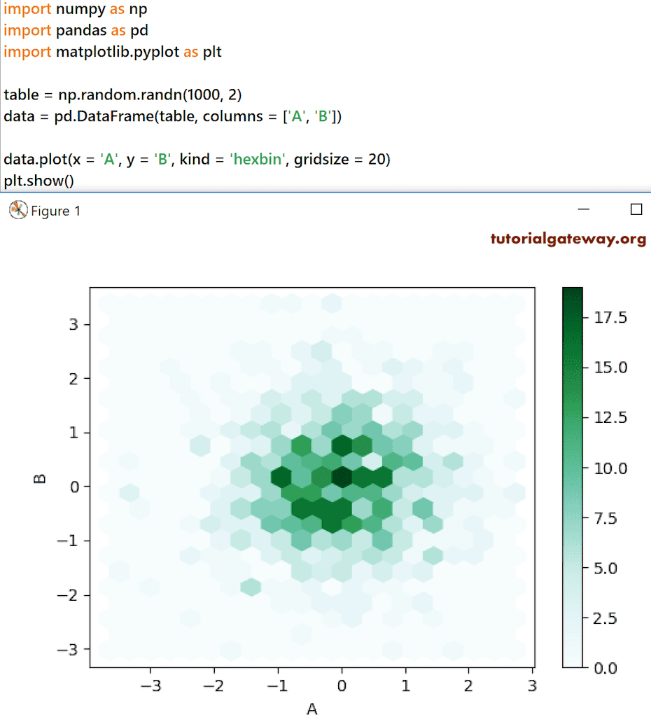
The hexbin plot is to generate a hexagonal binning plot.
First, we used Numpy random randn function to generate random numbers of size 1000 * 2. Next, we used the DataFrame function to convert that to a DataFrame with column names A and B. data.plot(x = ‘A’, y = ‘B’, kind = ‘hexbin’, gridsize = 20) creates a hexbin or hexadecimal bin graph using those random values.
import numpy as np
import pandas as pd
import matplotlib.pyplot as plt

table = np.random.randn(1000, 2)
data = pd.DataFrame(table, columns = ['A', 'B'])

data.plot(x = 'A', y = 'B', kind = 'hexbin', gridsize = 20)
plt.show()
Currently, we don’t have better data in our current table to display the hexadecimal bin plot. So, we used Sales 2018 vs. 2017 with grid size = 25.
import pyodbc
import pandas as pd
import matplotlib.pyplot as plt

conn = pyodbc.connect('''Driver={SQL Server Native Client 11.0}; Server=PRASAD; Database=SQL Tutorial ; Trusted_Connection=yes;''')

string = ( ''' SELECT Sales2018, Sales2017, Orders FROM EmployeeSales''')
query = pd.read_sql_query(string, conn)
df = pd.DataFrame(query)

df.plot.hexbin(y = 'Sales2018', x = 'Sales2017',gridsize = 25,  title = 'Hexbin Plot')
plt.show()

Histogram
The Python pandas DataFrame hist plot is to draw or generate a histogram of distributed data. In this example, we generated random values for x and y columns using the random randn function. Next, we used the Pandas hist function, not generating a histogram in Python.
import numpy as np
import pandas as pd
import matplotlib.pyplot as plt

A= np.random.randn(1000)
B= np.random.randn(1000) + 1
data = pd.DataFrame({'x':A, 'y': B}, columns = ['x', 'y'])

data.plot.hist()
plt.show()

This time we changed the total number of bins to 10 and added one more column to the DataFrame.
A= np.random.randn(1000)
B= np.random.randn(1000) + 1
C= np.random.randn(1000) - 2
data = pd.DataFrame({'x':A, 'y': B, 'z': C}, columns = ['x', 'y', 'z'])

data.plot.hist(bins = 10)
plt.show()

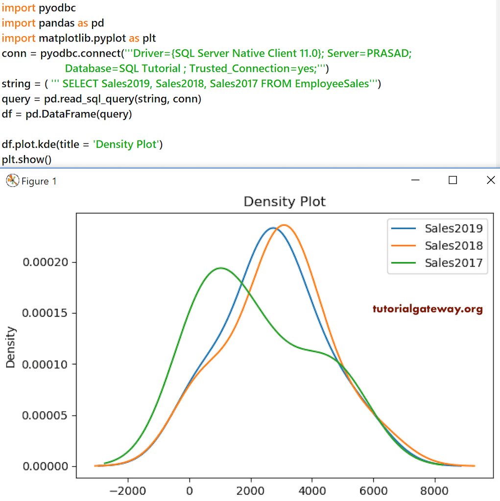
DataFrame kde plot
The Python pandas DataFrame kde generates or plots the Kernel Density Estimate chart (in short kde) using Gaussian Kernels. First, we used the Numpy random function to generate random numbers of size 10. Next, we are using the Pandas Series function to create a Series using those numbers. Finally, data.plot(kind = ‘kde’) generates a kde or density plot using that numbers.
table = np.random.randn(10)
data = pd.Series(table)
print(data)

data.plot(kind = 'kde')
plt.show()

Let me draw a density plot for the last three years of Sales in the Employees table DataFrame.
conn = pyodbc.connect('''Driver={SQL Server Native Client 11.0}; Server=PRASAD;
                      Database=SQL Tutorial ; Trusted_Connection=yes;''')

string = ( ''' SELECT Sales2019, Sales2018, Sales2017 FROM EmployeeSales''')
query = pd.read_sql_query(string, conn)

df = pd.DataFrame(query)
df.plot.kde(title = 'Density Plot')
plt.show()
Python Pandas DataFrame Line chart
The Line plot is to plot lines from a given data. You can use this line DataFrame to draw one dimension against single or multiple measures. Here, we drew the Pandas line for employee education against the Orders.
import pyodbc
import pandas as pd
import matplotlib.pyplot as plt
conn = pyodbc.connect('''Driver={SQL Server Native Client 11.0}; Server=PRASAD;
                      Database=SQL Tutorial ; Trusted_Connection=yes;''')
string = ( ''' SELECT EmpID ,FirstName, LastName ,Education, Occupation, YearlyIncome,
                    Sales2019, Sales2018, Sales2017, Orders FROM EmployeeSales''')
query = pd.read_sql_query(string, conn)
df = pd.DataFrame(query)

groupby_Occ = df.groupby('Education')['Orders'].sum()
groupby_Occ.plot(x = 'Education', y = 'Orders', kind = 'line',
                 title = 'Orders Vs Education  Line', legend = False)
plt.show()

We are grouping Education by Sales 2019, 2018, and 2017. Next, we have drawn a line chart using the line function. You can also use subplots = True inside the line function to separate those Sales lines.
groupby_Occ = df.groupby('Education')['Sales2019', 'Sales2018', 'Sales2017'].sum()
groupby_Occ.plot.line(title = 'Sales Vs Education  Line')
plt.show()

DataFrame Pie Chart
The Python pandas DataFrame plot Pie is to draw a pie chart. It slices a pie based on the numeric data column passed to it. Here, we generated a Pie chart using plot method where x = Occupation and y = Sales2019.
import pyodbc
import pandas as pd
import matplotlib.pyplot as plt
conn = pyodbc.connect('''Driver={SQL Server Native Client 11.0}; Server=PRASAD;
                      Database=SQL Tutorial ; Trusted_Connection=yes;''')
string = ( ''' SELECT EmpID ,FirstName, LastName ,Education, Occupation, YearlyIncome,
                    Sales2019, Sales2018, Sales2017, Orders FROM EmployeeSales''')
query = pd.read_sql_query(string, conn)
df = pd.DataFrame(query)

groupby_Occ = df.groupby('Occupation')['Sales2019'].sum()
groupby_Occ.plot(x = 'Education', y = 'Orders', kind = 'pie',
                 title = 'Sales Vs Occupation Pie Chart', legend = True)
plt.show()

Python Pandas DataFrame Scatter plot
The DataFrame Scatter plot creates or marks based on the given data. Each mark defines the coordinates of X and Y-axis values from a DataFrame.
conn = pyodbc.connect('''Driver={SQL Server Native Client 11.0}; Server=PRASAD;
                      Database=SQL Tutorial ; Trusted_Connection=yes;''')
string = ( ''' SELECT EmpID ,FirstName, LastName ,Education, Occupation, YearlyIncome,
                    Sales2019, Sales2018, Sales2017, Orders FROM EmployeeSales''')
query = pd.read_sql_query(string, conn)
df = pd.DataFrame(query)

df.plot(x = 'EmpID', y = 'Sales2017', kind = 'scatter')
plt.show()

Here, we used the X-axis value as EmpID and y as Sales 2019. Next, we changed the color of the dots to green and the size as well.
df.plot.scatter(x = 'EmpID', y = 'Sales2019', title = 'Scatter Plot',c = 'green', s = 24)
plt.show()
