The Vector is the most basic Data structure in R programming. A Vector can hold a collection of similar types of elements (type may be an integer, double, char, Boolean, etc.) If you type different data types in a single vector, then all the elements will be converted to a single type.
In this article, we show how to Create a Vector and how to access and manipulate the Elements. Next, Performing Arithmetic Operations on vectors.
Create a Vector in R
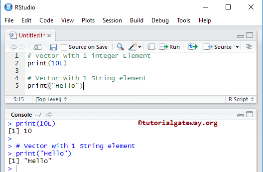
Every variable will be internally converted to Vector. In this example, we will create a vector in this programming of a single element. The most basic way to create is.
# with 1 integer Element
print(10L)

# with 1 String element
print("Hello")
Create R Vector using Range
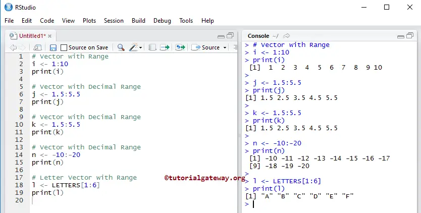
In this programming, there is a special operator called Range or Colon, and this will help to create a vector. For example, i <- 1:10 means 1, 2, 3, 4, 5, 6, 7, 8, 9, 10
# with Range
i <- 1:10
print(i)

# with Decimal Range
j <- 1.5:5.5
print(j)

# with Decimal Range
k <- 1.5:5.5
print(k)

# with Decimal Range
n <- -10:-20
print(n)

# Letter with Range
l <- LETTERS[1:6]
print(l)
Create R Vector using Sequence (seq) Operator
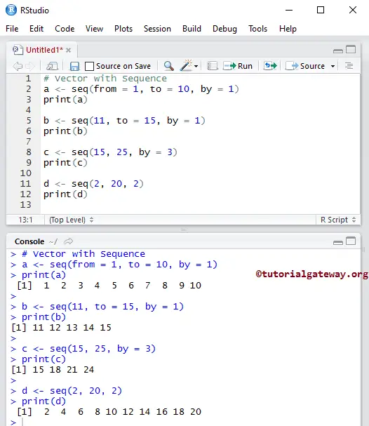
Here, we create a vector in this programming using a sequence operator or simply a seq operator. The Sequence operator will return values sequentially.
# with Sequence
a <- seq(from = 1, to = 10, by = 1)
print(a)

# Here, from =, to =, by = values are option so you can remove them too
b <- seq(11, to = 15, by = 1) # Removing from
print(b)

c <- seq(15, 25, by = 3) # Removing both from, to
print(c)

d <- seq(2, 20, 2) # removing from, to, and by
print(d)
It will create a Vector starting with Value 1 at index position 1 and ending with Value 10 at index position 10 by incrementing the value by 1. It means 1, 2, 3, 4, 5, 6, 7, 8, 9, 10
a <- seq(from = 1, to = 10, by = 1)
Creating R Vector using concatenation c
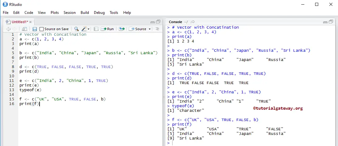
This example creates a vector using c, or we say concatenation. It is the most popular R Programming approach, and normally we prefer this way.
# with Concatenation

# Numeric
a <- c(1, 2, 3, 4)
print(a)

# Character
b <- c("India", "China", "Japan", "Russia", "Sri Lanka")
print(b)

#Boolean
d <- c(TRUE, FALSE, FALSE, TRUE, TRUE)
print(d)

# Mixed and its Type will be Character
e <- c("India", 2, "China", 1, TRUE)
print(e)
typeof(e) # this will return the Data type of e

# Placing or Nesting One inside the another
f <- c("UK", "USA", TRUE, FALSE, b) # b is another one
print(f)
Access R Vector Elements
In this programming, We can use the index position to access the elements in a Vector. Using this index value, we can access or alter/change each and every individual element present. The index value starts at 1 and ends at n where n is the length.
For example, if we declare a vector that stores 10 elements, then the index starts at 1 and ends at 10. To access or alter the 1st value, use Vector_Name[1], and to alter or access the 10th value, use Vector_Name[10].
# Elements Accessing
a <-  c("India", "China", "Japan", "UK", "USA", "Russia", "Sri Lanka")
print(a)

print(a[1])
print(a[3])

print(a[1:3])
print(a[4:6])
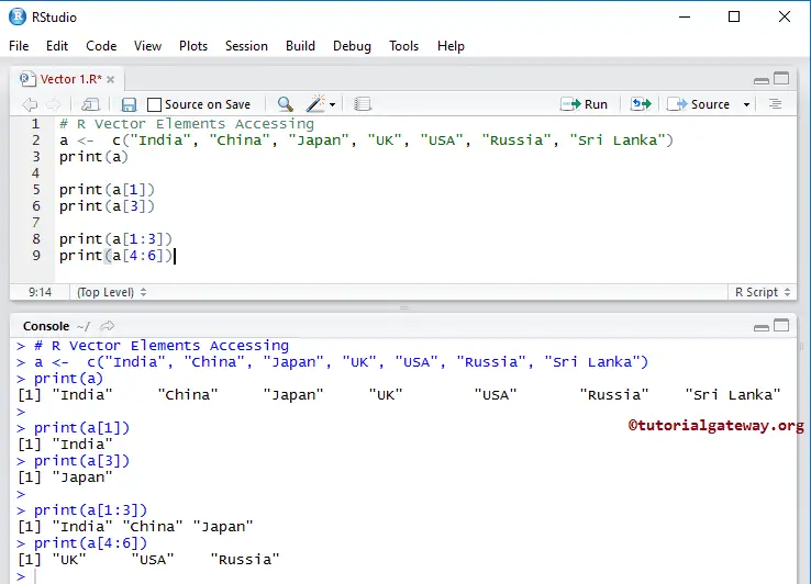
First, we declared a R Vector called a and assigned the following values
a <- c("India", "China", "Japan", "UK", "USA", "Russia", "Sri Lanka")
Here, a[1] means element at the first position (i.e., India), and a[3] means element at the third position (i.e., Japan).
print(a[1])
print(a[3])
In the next line, we used the special operator Range (or Colon). It prints the elements from 1 through 3 (i.e., 1, 2, 3)
print(a[1:3])
Access using Vector
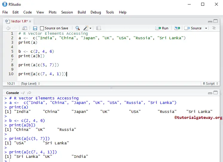
This example accesses the elements using another Vector. In the sixth line print(a[b]), we used those numbers as the index position to access the elements. It means prints the elements at index positions 2, 4, and 6.
# Elements Accessing
a <-  c("India", "China", "Japan", "UK", "USA", "Russia", "Sri Lanka")
print(a)

b <- c(2, 4, 6)
print(a[b])

print(a[c(5, 7)])

print(a[c(7, 4, 1)])
Using Negative Values in R Vector
Accessing the elements using Negative values and Boolean values. In Vectors, the Negative index position is used to omit those values.
# Elements Accessing
a <-  c("India", "China", "Japan", "UK", "USA", "Russia", "Sri Lanka")
print(a)

b <- c(-3, -7)
print(a[b])

print(a[c(-4, -6, -7)])

print(a[c(TRUE, FALSE, TRUE, TRUE, FALSE, TRUE, FALSE)])
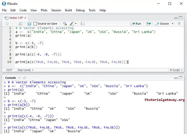
First, we declared b of negative numbers -3 and -7.
b <- c(-3, -7)
In the next line, we used those numbers as the index position to access the elements. It means printing the elements except for the values at index positions 3 and 7.
print(a[b])
In the next line, we declared a Boolean. We used those Boolean values as the index position to access elements. Here, TRUE means print the value, and FALSE means don’t print. It means print elements at positions 1, 3, 4, 6.
print(a[c(TRUE, FALSE, TRUE, TRUE, FALSE, TRUE, FALSE)])
Use Character Vectors as Index
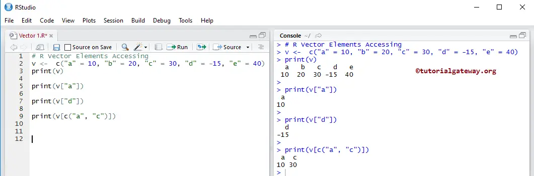
This example shows how to access the R Vector elements using Character Index values. Here, we declare v with alphabet indexes that can help us extract the elements using the alphabet.
v <-  c("a" = 10, "b" = 20, "c" = 30, "d" = -15, "e" = 40)
print(v)

print(v["a"])

print(v["d"])

print(v[c("a", "c")])
Manipulate Vector Elements
In this Programming, we can manipulate the Vector elements in the following ways:
# Elements Manipulation
a <-  c(10, 20, 30, -15, 40, -25, 60, -5)
print(a)

a[7] <- 77
print(a)

a[a < 0] <- 99
print(a)

# Truncating the Elements
a <- a[1:5]
print(a)

# Deleting
a <- NULL
print(a)
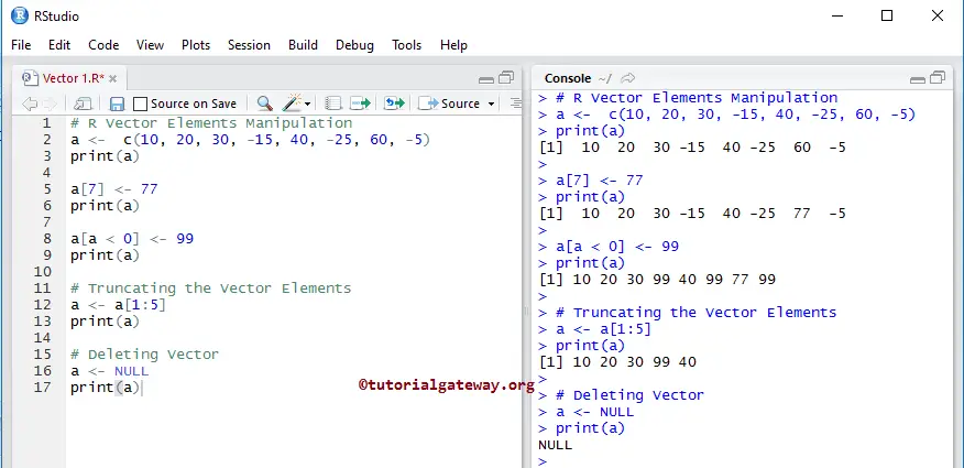
Assigning 77 at position 7.
a[7] <- 77
It will assign 99 to all the elements whose values are less than 0. Here a < 0 will check whether the element is less than zero or not, and if the condition is true, then that element will be replaced by 99.
a[a < 0] <- 99
In vector Slicing, the first integer value is the index position where the slicing will start, and the second is the index position of the slicing will end.
a <- a[1:5]
It removes a complete.
a <- NULL
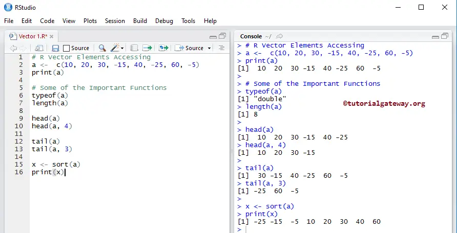
Important Functions of Vector in R
The following functions are some of the most useful functions supported by the Vectors in this programming.
- typeof(VectorName): Returns the data type.
- Sort(Vector_name): Sort the items in Ascending order.
- length(Vector_name): Counts the number of items.
- head(Vector_name, limit): Returns the top six items (if you Omit the limit). If you specify the limit as 4, then it returns the first 4 items.
- tail(Vector_name, limit): It returns the last six items (if you Omit the limit). If you specify the limit as 2, then it returns the last two items.
# Elements Accessing
a <-  c(10, 20, 30, -15, 40, -25, 60, -5)
print(a)

# Some of the Important Functions
typeof(a)
length(a)

head(a)
head(a, 4)

tail(a)
tail(a, 3)

x <- sort(a)
print(x)
Arithmetic Operations on Vector
Using Arithmetic Operators to perform arithmetic operations.
a <-  c(10, 20, 30, 40)
b <-  c(12, 26, 38, 44)

print(a + b)

print(b - a)

print(a * b)

print (2 * a)

d <- c(12, 44)
print(a + d)
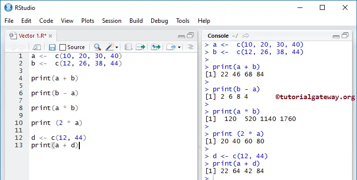
First, we declared two numeric an and b of the same length. Next, we performed addition, subtraction, and multiplication on these vectors. Here a + b means (10 + 12, 20 + 26, 30 + 38, 40 + 44) = (22, 46, 38, 44)
print(a + b)
print(b - a)
print(a * b)
The above things will work as long as the length is the same. But, if the lengths are different, then element recycling will happen. It will travel and multiply each item by 2 until it finishes the elements.
print (2 * a)
Next, we declared d of two elements and performed the addition. Here a + d means (10 + 12, 20 + 44, 30 + 12, 40 + 44) because we have only two items in d so those two items will be repeated.
d <- c(12, 44)
print(a + d)