SQL LAG Function

The SQL Server LAG function is one of the Analytic functions that act precisely opposite to LEAD. It allows you to access the data or value from a previous row without using any SELF JOIN. This SQL LAG function is beneficial in comparing the current row value with its previous row.

The values returned by the LAG Function depend on the ORDER BY clause. The ORDER BY clause decides the sorting of numeric values, and the LAG function retrieves the previous row in the same order. This article will explore the SQL Server LAG function Partitioned by clause and Default and Offset Values.

SQL LAG Function Syntax

The basic syntax of the SQL LAG function is as shown below:

SELECT LAG([Scalar Expression], [Offset_Value], [Default_Value]) 
                  OVER (
                         PARTITION_BY_Clause 
                         ORDER_BY_Clause
                        )
FROM [Source]

Let us explore the Parameters of the SQL Server LAG Function.

Scalar Expression: It can be a Column Name, expression, or Subquery from which you want to retrieve the previous value. It returns a single value.
Offset_Value (Optional): Please define the number of rows you want to move or look backward from the current row. The default value = 1, so the SQL LAG function retrieves the previous row value. For example, if the Offset is 3, it looks back at three rows and will select the 3rd previous row (-3) value as a result set. Use a Column, Subquery, or any expression that returns a single value.
Default_Value (Optional): It allows you to define the default value and accepts a constant value or an expression. This default value will return if the previous row value is NULL or the Offset_Value is not in the range. If you ignore it, NULL will return.
Order_By_Clause: Please specify the column name to sort the partitioned data in Ascending or Descending order. Please refer to Order By Clause in SQL Server.
Partition_By_Clause: It separates the Selected records result set into partitions based on the given column. For instance, partition employees by department name.
- If you specify the Partition By Clause, the SQL Server LAG function works independently within each partition. It starts picking the previous rows in each partition and does the same for other partitions.
- If the partition By clause is not specified, the LAG function will consider all table rows as a single partition.

SQL Server LAG function Examples

This section will explore the SQL LAG function to retrieve previous rows and what happens when we ignore the Partition By Clause. We will use the below-shown Employee table data for this LAG function demonstration.

SQL LAG Function without a Default Value

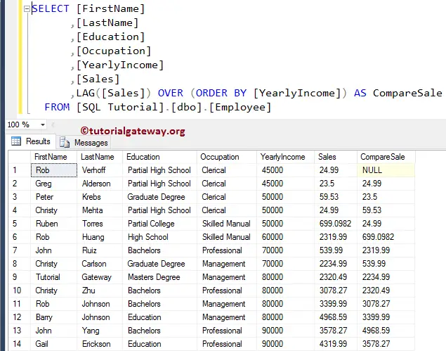
The below query is a simple and basic example of the LAG function. We did not use the Offset, Default Value, and Partition By Clause to retrieve the previous sales. As we didn’t use the Partition By, the SQL LAG function considers the whole table a single partition.

The ORDER BY [YearlyIncome] statement sorts the Employee records in Ascending order based on their Yearly Income. Next, LAG([Sales]) will return the previous Sales value of the row (record before) as the output. If there are no rows to return, the SQL Server LAG function will return a NULL value because we haven’t set any default value.

SELECT [FirstName]
      ,[LastName]
      ,[Education]
      ,[Occupation]
      ,[YearlyIncome]
      ,[Sales]
      ,LAG([Sales]) OVER (ORDER BY [YearlyIncome]) AS CompareSale 
  FROM [Employee]

As you can see, the SQL LAG function returned NULL as output for the 1st record. It’s because there is no previous row for that record (it is the first record, indeed). The second record of the CompareSale column is the first-row value of the Sales column.

SQL Server LAG Function with a default value

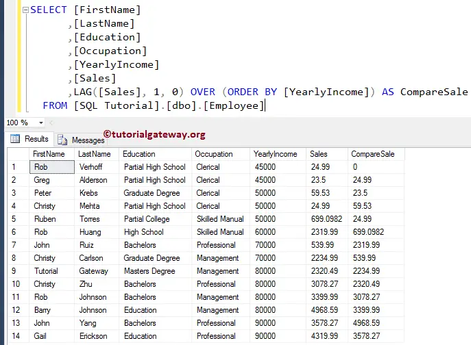
The SQL LAG function provides flexibility to specify a default value that will return when no data is in the previous row. If you observe the above image, the first row of the CompareSale column is NULL. So, let me define the Offset value = 1 and the default value = 0.

SELECT [FirstName]
      ,[LastName]
      ,[Education]
      ,[Occupation]
      ,[YearlyIncome]
      ,[Sales]
      ,LAG([Sales], 1, 0) OVER (ORDER BY [YearlyIncome]) AS CompareSale 
FROM [Employee]

You can see that the LAG function is replacing the CompareSale column NULL value with 0. Please refer to the LEAD and SELF JOIN articles.

Offset value =1, and the default value = 0

SQL LAG Function with Partition By Clause

How to write the previous values from the partitioned records is one of the common questions you may face in interviews. The PARTITION BY clause divides the table into multiple partitions based on a specified column.

The following query partitions the Employee table data by Occupation, which means each unique occupation type is a separate partition. The ORDER BY [YearlyIncome] line sort each partition using their employee’s yearly Income. And then, the SQL LAG function returns previous Sales values in each partition (employee occupation). The server will reset the LAG value when it goes to the subsequent Occupation.

SELECT [FirstName] + ' ' + [LastName] AS [Full Name]
      ,[LastName]
      ,[Education]
      ,[Occupation]
      ,[YearlyIncome]
      ,[Sales]
      ,LAG([Sales], 1, 0) OVER (
   PARTITION BY [Occupation]
   ORDER BY [YearlyIncome]
 ) AS SaleCompare 
FROM [Employee]

If you see, for the 1st, 5th, 9th, and 13th records, the SQL LAG function is assigned 0 because there are no previous records within that partition. If you remove the default value, those 0’s will replace by NULLs.

SQL Server LAG Function with Partition By Clause Example

SQL LAG Function with Offset Value 2

In the above statement, we used the SQL LAG function with partition by clause, and it selected the previous rows with the individual partition. It is because, By default, the LAG function returns the value from the previous row. However, you can also specify the offset value.

Let us see what happens when we change the SQL LAG Function offset value from 1 to 2 and the default value to 100.

SELECT [FirstName] + ' ' + [LastName] AS [Full Name]
      ,[Education]
      ,[Occupation]
      ,[YearlyIncome]
      ,[Sales]
      ,LAG([Sales], 2, 100) OVER (
   PARTITION BY [Occupation]
   ORDER BY [YearlyIncome]
          ) AS SaleCompare  
FROM [Employee]

As you can see, we used an offset of 2, and this SQL LAG function selects the -2nd row (2 rows ahead) rather than the previous row. Modifying the offset value to 3 will look three rows back and select the last third row (-3rd row) by jumping the last two rows, etc.